Three Bus Pricing

Last updated for Convexity v0.4.3

This tutorial shows the price dynamics of a three-bus system to illustrate visualisation options in Convexity.

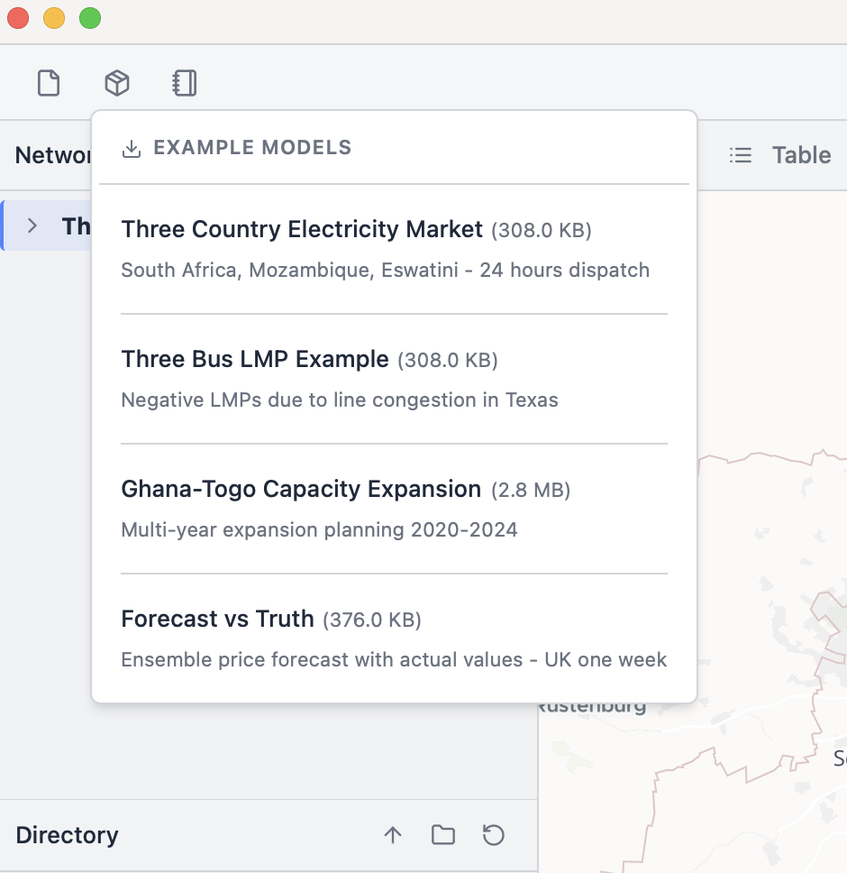
You can open the example model for this tutorial by by clicking on the cube icon in the top-left of the app and selecting "Three Bus LMP Example":

The example models menu

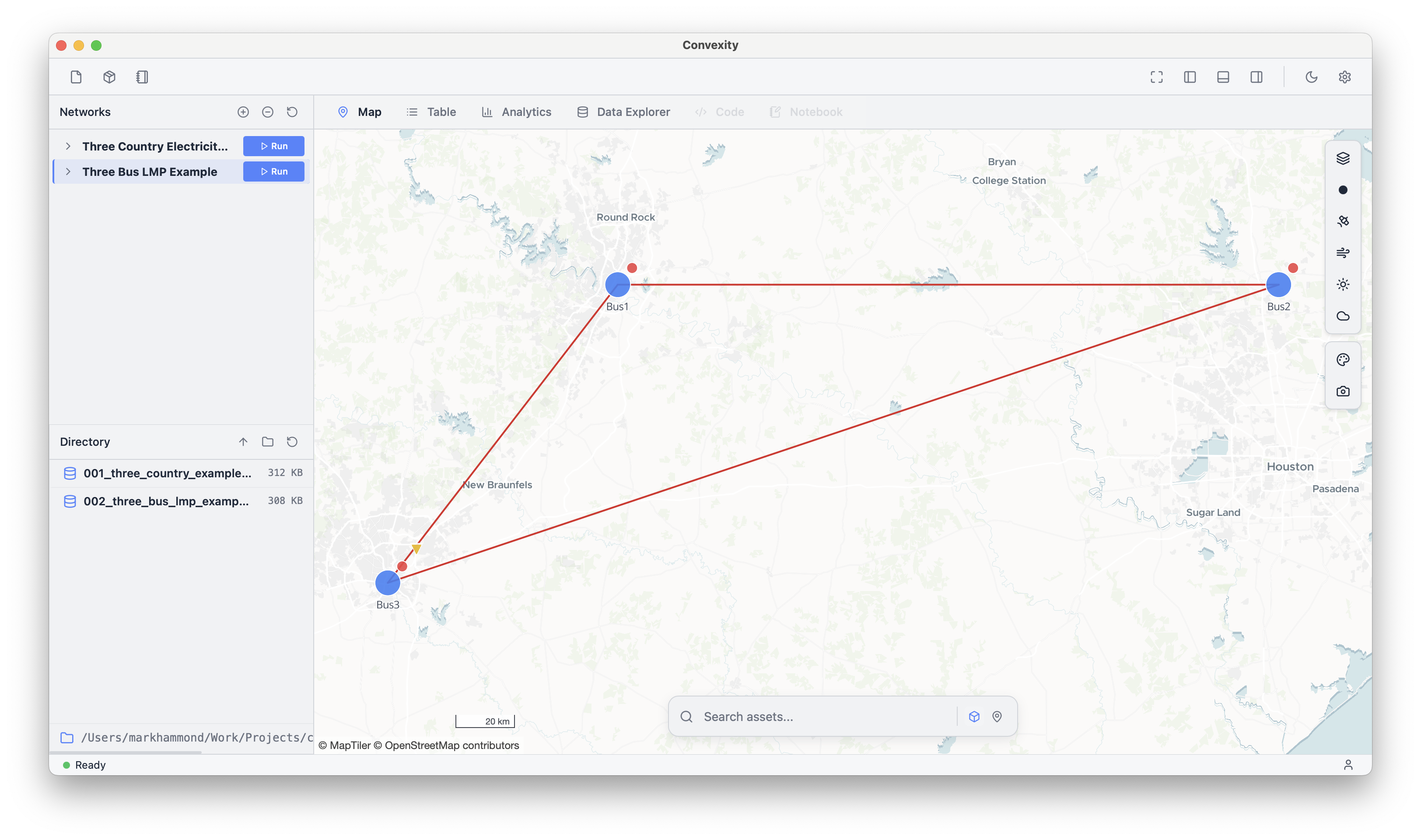
This example has three buses like the first example, and is inspired by this 3 Bus LMP model. This tutorial will show how to view and edit charts of the model results, and discuss what they show about dispatch patterns and pricing.

The Three Bus Pricing model open in the Convexity app

You can view the attributes of each component either by clicking on it on the map, or by going to the Table tab and selecting a component type from the dropdown in the top left, such as Generators:

The table of generators in the model, one on each bus

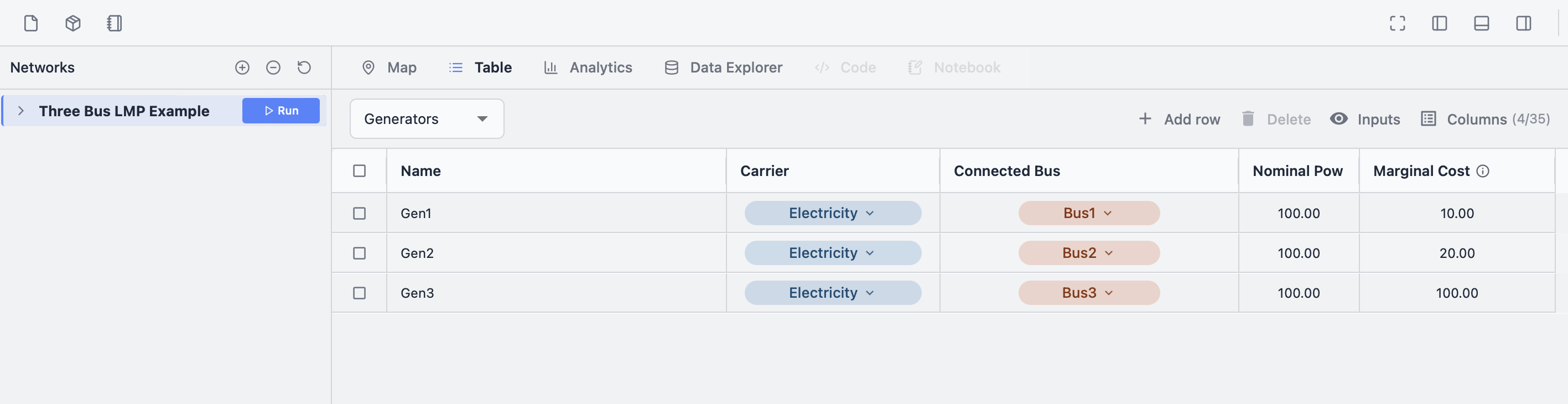
This shows that we have three 100 MW generators in the network, one on each bus, with different marginal prices.

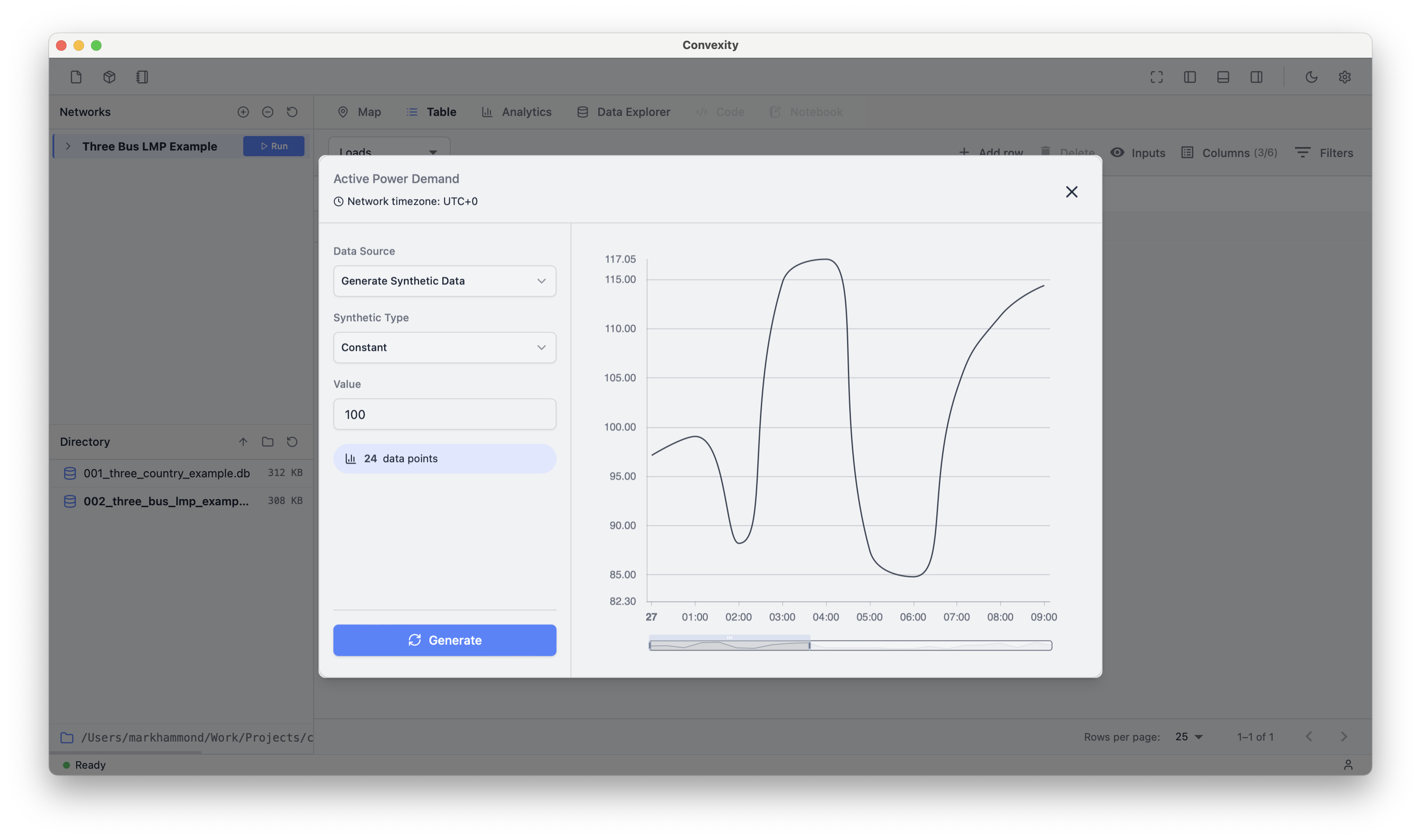
We can inspect the load in the model by selecting "Loads" in the table tab, where we see that there is just one load attached to Bus 3:

The table of loads in the model, showing that there is just one

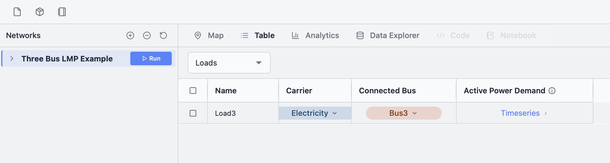
Unlike the static values for the generator capacities, the load has a time-varying demand shown as "Timeseries". Clicking on that text opens a plot of the timeseries:

The timeseries viewer for the demand of the load on Bus 3

You can open the Lines table to see that there are three lines in the model, connecting the buses in a triangle, wth capacities:

1. Bus 1 to 2: 100 MW
2. Bus 1 to 3: 10 MW
3. Bus 2 to 3: 100 MW

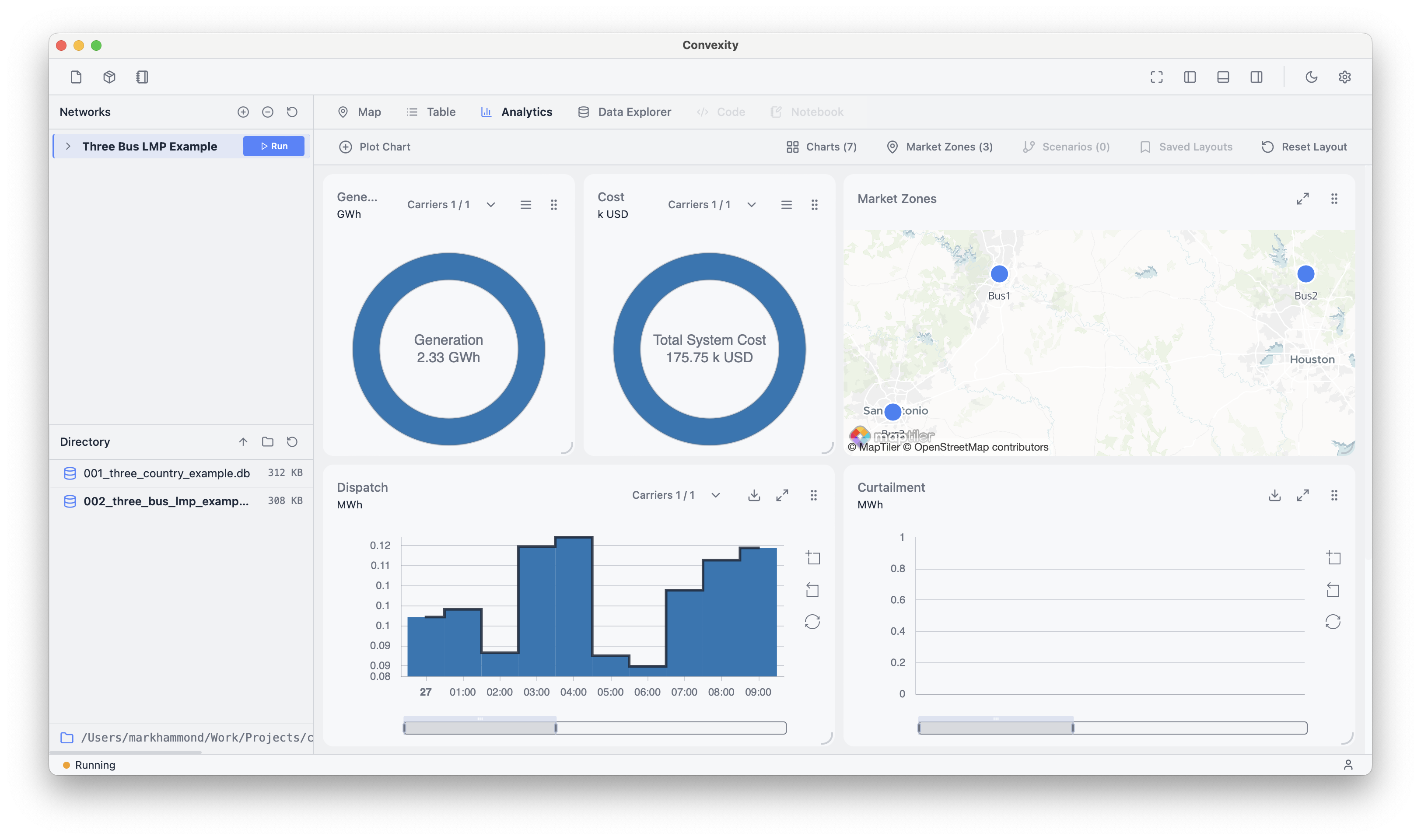
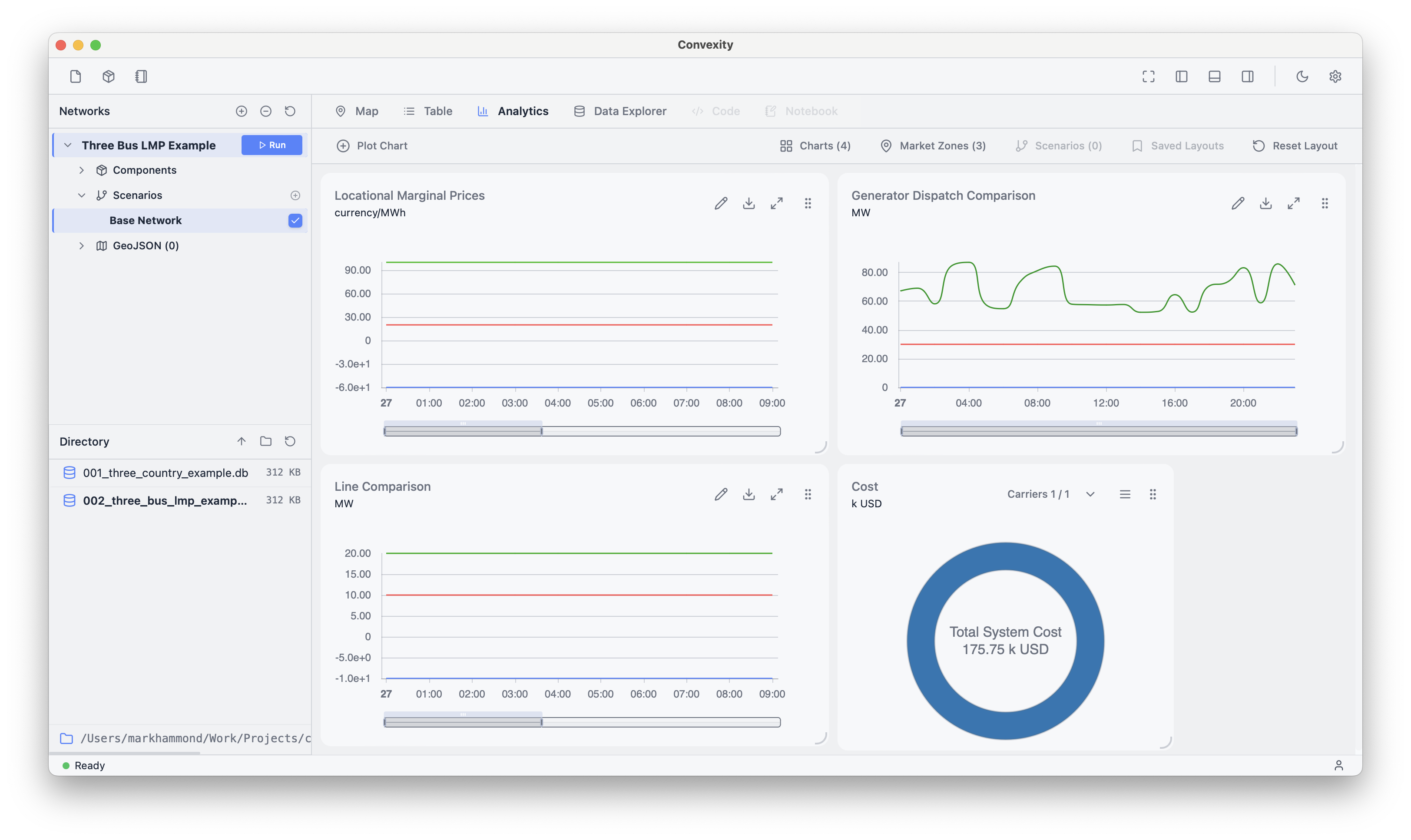
These limited line sizes will lead to interesting pricing dynamics. Press "Run" next to the network name in the tree view in the top left, to start the solve running in the bottom tab. Once it's complete, open the Analytics tab to view to see how the time-varying load is satisfied by the generic "Electricity" generators:

The analytics tab for this example model

We'll now make a custom plot to view the price at each bus. Click "Plot Chart" in the top left of the analytics tab to open up the chart editor:

The chart editor in the analytics tab, showing locational marginal price per bus

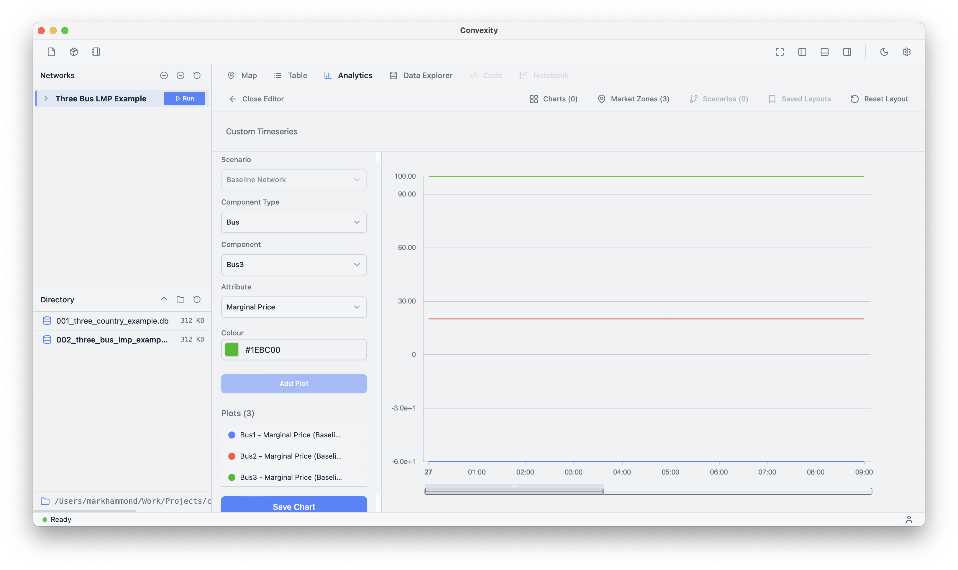
Here, we've selected the marginal price attribute for each bus in the model. Clicking "Save Chart" saves the chart to the main analytics dashboard. Bus 1, 2, and 3 have marginal prices of -60, 20, and 100 £/MWh respectively.

This shows how locational marginal prices depend on both generator marginal prices, and transmission constraints. We can inspect the dynamics by creating a plot of the dispatch per generator:

The analytics tab, showing dispatch by each generator at each bus, and the resulting marginal price at each bus

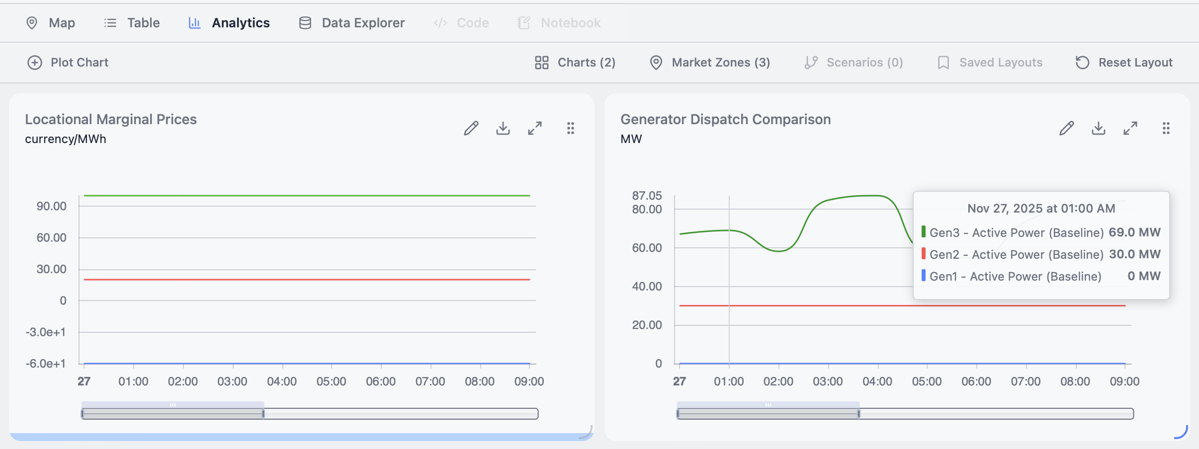
This shows how transmission constraints have led to the cheapest generator (Generator 1) not being dispatched at all. This is because the lines are operating at their maximum capacity:

The analytics tab, with the power flow over each line shown in the bottom left.

This leads to the negative marginal price at Bus 1, which implies that increasing demand at that bus will reduce total system cost (as oppposed to a typical positive marginal price, where increasing demand increases total cost).

We can see this by adding a 1 MW load to Bus 1 (right-clicking on the map, selecting "Add Load", and setting it to 1 MW) and re-solving the model:

The results of adding an extra 1 MW load to Bus 1 -- total system cost decreases.

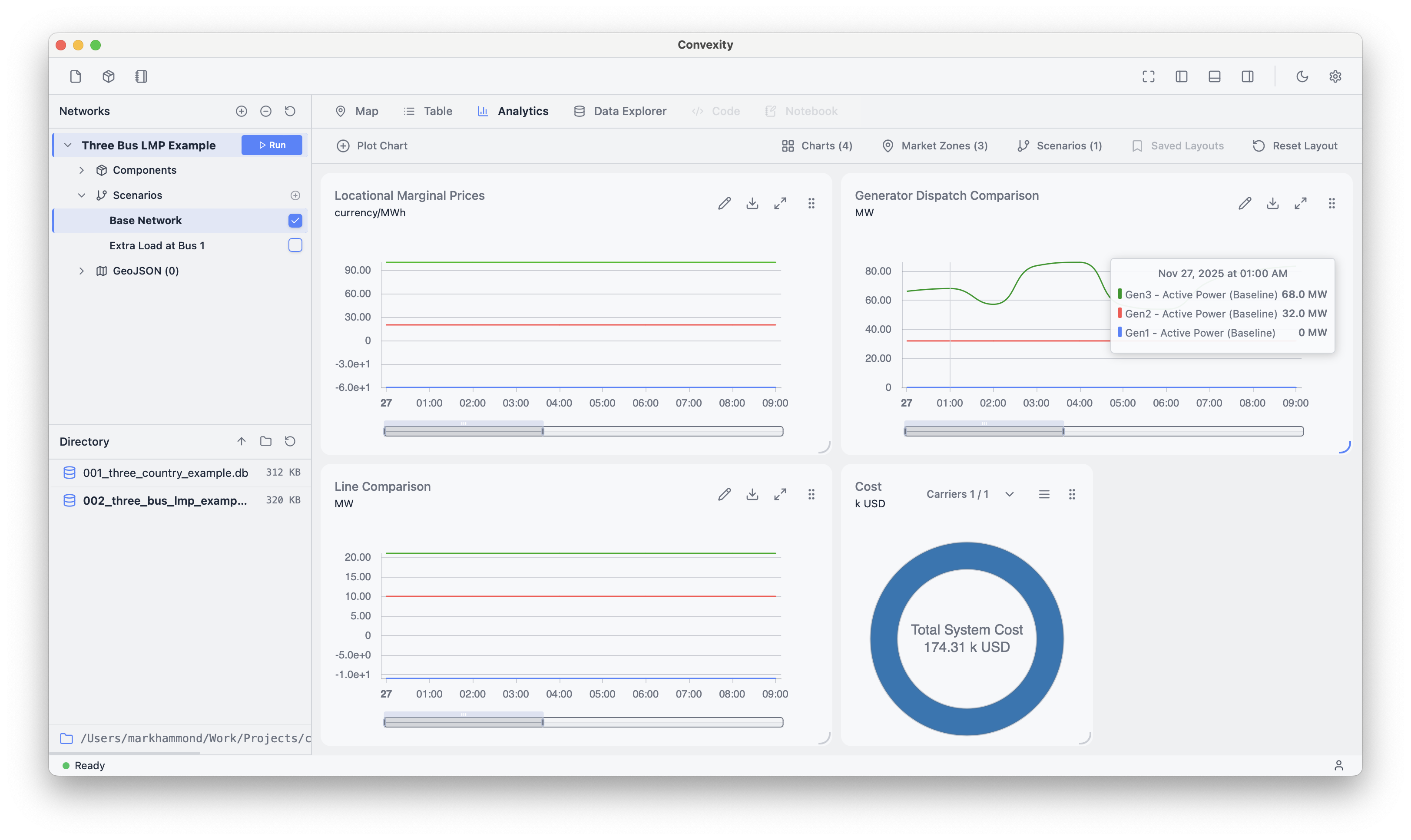
We can see that the total system cost decreases from 175.75k to 174.31k.

This surprising result is because adding an extra load at Bus 1 decreases the net flow from Bus 1 to Bus 3. This allows Generator 2 to provide an additional 2 MW dispatch to Bus 1 (see above plots), with 1 MW of that satisfying the demand at Bus 1, and 1 MW of it flowing onwards to Bus 3.

This allows Generator 3 -- the most expensive at 100 marginal cost -- to dispatch 1 MW less than before, which is instead provided by Generator 2 at 20 marginal cost, reducing the total cost of the system.